Trust Region Policy Optimization
Thank you to Nic Ford, Ethan Holly, Matthew Johnson, Avital Oliver, John Schulman, George Tucker, and Charles Weill for contributing to this guide.
Why
TRPO is a scalable algorithm for optimizing policies in reinforcement learning by gradient descent. Model-free algorithms such as policy gradient methods do not require access to a model of the environment and often enjoy better practical stability. Consequently, while straightforward to apply to new problems, they have trouble scaling to large, nonlinear policies. TRPO couples insights from reinforcement learning and optimization theory to develop an algorithm which, under certain assumptions, provides guarantees for monotonic improvement. It is now commonly used as a strong baseline when developing new algorithms.
1 Policy Gradient
Motivation: Policy gradient methods (e.g. TRPO) are a class of algorithms that allow us to directly optimize the parameters of a policy by gradient descent. In this section, we formalize the notion of Markov Decision Processes (MDP), action and state spaces, and on-policy vs off-policy approaches. This leads to the REINFORCE algorithm, the simplest instantiation of the policy gradient method.
Topics:
- Markov Decision Processes.
- Continuous action spaces.
- On-policy and off-policy algorithms.
- REINFORCE / likelihood ratio methods.
Required Readings:
- Deep RL Course at UC Berkeley (CS 294); Policy Gradient Lecture
- David Silver’s course at UCL; Policy Gradient Lecture
- Reinforcement Learning by Sutton and Barto, 2nd Edition; pages 265 - 273
- Simple statistical gradient-following algorithms for connectionist reinforcement learning
Optional Readings:
- John Schulman introduction at MLSS Cadiz
- Lecture on Variance Reduction for Policy Gradient
- Introduction to policy gradient and motivations by Andrej Karpathy
- Connection Between Importance Sampling and Likelihood Ratio
Questions:
- At its core, REINFORCE computes an
approximate gradient of the reward with respect to the parameters. Why
can’t we just use the familiar stochastic gradient descent?
Hint
Just as in reinforcement learning, when we use stochastic gradient descent, we also compute an estimate of the gradient, which looks something like $$\nabla_{\theta} \mathbb{E}_{x \sim p(x)} [ f_{\theta}(x) ] = \mathbb{E}_{x \sim p(x)} [\nabla_{\theta} f_{\theta}(x)]$$ where we move the gradient into the expectation (an operation made precise by the Leibniz integral rule). In other words, the objective we're trying to take the gradient of is indeed differentiable with respect to the inputs. In reinforcement learning, our objective is non-differentiable -- we actually select an action and act on it. To convince yourself that this isn't something we can differentiate through, write out explicitly the full expansion of the training objective for policy gradient before we move the gradient into the expectation. Is sampling an action really non-differentiable? (spoiler: yes, but we can work around it in various ways, such as using REINFORCE or other methods).
- Does the REINFORCE gradient estimator resemble maximum likelihood estimation (MLE)?
Why or why not?
Solution
The term \( \log \pi (a | s) \) should look like a very familiar tool in statistical learning: the likelihood function! When we think of what happens when we do MLE, we are trying to maximize the likelihood of \( \log p(D | \theta) \) or as in supervised learning, we try to maximize $$\log p(y_i^* | x_i, \theta).$$ Normally, because we have the true label \( y_i^* \), this paradigm aligns perfectly with what we are ultimately trying to do with MLE. However, this naive strategy of maximizing the likelihood \( \pi(a | s) \) won't work in reinforcement learning, because we do not have a label for the correct action to be taken at a given time step (if we did, we should just do supervised learning!). If we tried doing this, we would find that we would simply maximize the probability of every action; make sure you convince yourself this to be true. Instead, the only (imperfect) evidence we have of good or bad actions is the reward we receive at that time step. Thus, a reasonable thing to do seems like scaling the log-likelihood by how good or bad the action by the reward. Thus, we would then maximize $$r(a, s) \log \pi (a | s).$$ Look familiar? This is just the REINFORCE term in our expectation: $$ \mathbb{E}_{s,a} [ \nabla r(a, s) \log \pi (a | s) ] $$
- In its original formulation, REINFORCE is an on-policy algorithm. Why?
Can we make REINFORCE work off-policy as well?
Solution
We can tell that REINFORCE is on-policy by looking at the expectation a bit closer: $$ \mathbb{E}_{s,a} [ \nabla \log \pi (a | s) r(a, s). ]$$ When we see any expectation in an equation, we should always ask what exactly is the expectation over? In this case, if we expand the expectation, we have: $$\mathbb{E}_{s \sim p_{\theta}(s), a \sim \pi_{\theta}(a|s)} [ \nabla_{\theta} \log \pi_{\theta} (a | s) r(a, s), ]$$ and we see that while the states are being sampled from the empirical state visitation distribution induced by the current policy, and the actions \( a \) are coming directly from the current policy. Because we learn from the current policy, and not some arbitrary policy, REINFORCE is an on-policy. To change REINFORCE to use data, we simply change the sampling distribution to some other policy \( \pi_{\beta} \) and use importance sampling to correct for this disparity. For more details, see a classic paper on this subject and a recent paper with new insights on off-policy learning with policy gradient methods.
- Do policy gradient methods work for discrete and continuous action spaces? If not, why not?
2 Variance Reduction and Advantage Estimate
Motivation: One major shortcoming of policy gradient methods is that the simplest instantation of REINFORCE suffers from high variance in the gradients it computes. This results from the fact that rewards are sparse, we only visit a finite set of states, and that we only take one action at each state rather than try all actions. In order to properly scale our methods to harder problems, we need to reduce this variance. In this section, we study common tools for reducing variance for REINFORCE. These include a causality result, baselines, and advantages. Note that the TRPO paper does not introduce new methods for variance reduction, but we cover it here for complete understanding.
Topics:
- Causality for REINFORCE.
- Baselines and control variates.
- Advantage estimation.
Required Readings:
- Deep RL Course at UC Berkeley (CS 294); Actor-Critic Methods Lecture
- George Tucker’s notes on Variance Reduction
Optional Readings:
- Reinforcement Learning by Sutton and Barto, 2nd Edition; pages 273 - 275
- High-dimensional continuous control using generalized advantage estimation
- Asynchronous Methods for Deep Reinforcement Learning
- Monte Carlo theory, methods, and examples by Art B. Owen; Chapter 8 (in-depth treatment of variance reduction; suitable for independent study)
Questions:
- What is the intuition for using advantages instead of rewards as the learning signal? Note on terminology: the learning signal is the factor by which we multiply \(\log \pi (a | s)\) inside the expectation in REINFORCE.
- What are some assumptions we make by using baselines as a variance reduction method?
- What are other methods of variance reduction?
Solution
Check out the optional reading Monte Carlo theory, methods, and examples by Art B. Owen; Chapter 8 if you're interested! Broadly speaking, other techniques for doing variance reduction for Monte Carlo integration include stratified sampling, antithetic sampling, common random variables, conditioning.
- The theory of control variates tells us that our control variate should
be correlated with the quantity we are trying to lower the variance of.
Can we construct a better control variate that is even more correlated
than a learned state-dependent value function? Why or why not?
Hint
Right now, the typical control variate \( b(s) \) depends only on the state. Can we also have the control variate depend on the action? What extra work do we have to do to make sure this is okay? Check this paper if you're interested in one way to extend this, and this paper if you're interested in why adding dependence on more than just the state can be tricky and hard to implement in practice.
- We use control variates as a method to reduce variance in our gradient
estimate. Why don’t we use these for supervised learning problems such as
classification? Are we implicitly using them?
Solution
Reducing variance in our gradient estimates seems like an important thing to do, but we don't often see explicit variance reduction methods when we do supervised learning. However, there is a line of work around stochastic variance reduced gradient descent called SVRG that tries to construct gradient estimators with reduced variance. See these slides and these papers for more on this topic.
The reason that we don't often see these being used in the supervised learning setting is because we're not necessarily looking to reduce the variance of SGD and smoothly converge to a minima. This is because we're actually interested in looking for minima that have low generalization error and don't want to overfit to solutions with very small training error. In fact, we often rely on the noise introduced by using minibatches in SGD to help us to escape premature minima. On the other hand, in reinforcement learning, the variance of our gradient estimates is so high that it's often the foremost problem.
Beyond supervised learning, control variates are used often in Monte Carlo integration, which is ubiquitous throughout Bayesian methods. They are also used for problems in hard attention, discrete latent random variables, and general stochastic computation graphs.
3 Fisher Information Matrix and Natural Gradient Descent
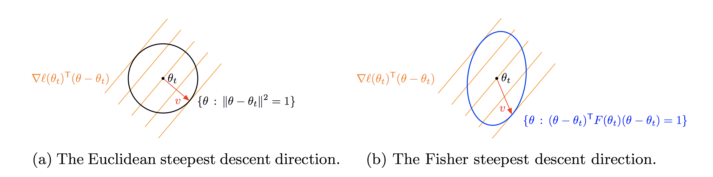
Motivation: While gradient descent is able to solve many optimization problems, it suffers from a basic problem - performance is dependent on the model’s parameterization. Natural gradient descent, on the other hand, is invariant to model parameterization. This is achieved by multiplying gradient vectors by the inverse of the Fisher information matrix, which is a measure of how much model predictions change with local parameter changes.
Topics:
- Fisher information matrix.
- Natural gradient descent.
- (Optional) K-Fac.
Required Readings:
- Matt Johnson’s Natural Gradient Descent and K-Fac Tutorial: Sections 1-7, Section A, B
- New insights and perspectives on the natural gradient method: Sections 1-11.
- Fisher Information Matrix
Optional Readings:
- 8-page intro to natural gradients
- Why Natural Gradient Descent / Amari and Douglas
- Natural Gradient Works Efficiently in Learning / Amari
Questions:
- Consider classifiers \(p(y | x; \theta_{1})\) and \(p(y | x; \theta_{2})\),
such that \(l_2(\theta_1, \theta_2)\) is large, where \(l_2\) indicates the
Euclidean distance metric. Does this imply the difference in accuracy of the
classifiers is high?
Solution
The accuracy of the classifier depends on the function defined by \(p(y|x;\theta) \). The distance between the parameters do not inform us about distance between the two functions. Hence, we cannot draw any conclusions about the difference in accuracy of the classifiers. - How is the Fisher matrix similar and different from the Hessian?
- How does natural gradient descent compare to Newton’s method?
- Why is the natural gradient slow to compute?
- How can one efficiently compute the product of the Fisher information matrix with an arbitrary vector?
4 Conjugate Gradient
Motivation: The conjugate gradient method (CG) is an iterative algorithm for finding approximate solutions to \(Ax=b\), where \(A\) is a symmetric and positive-definite matrix (such as the Fisher information matrix). The method works by iteratively computing matrix-vector products \(Ax_i\) and is particularly well-suited for matrices with computationally tractable matrix-vector products.
Topics:
- Solving system of linear equations.
- Efficiently computing matrix-vector products.
- Computational complexities of second order methods optimization methods.
Required Readings:
- An Introduction to the Conjugate Gradient Method Without the Agonizing Pain: Section 7-9
- Convex Optimization and Approximation, UC Berkeley, Section 7.4
- Convex Optimization II by Stephen Boyd:
Optional Readings:
- Numerical Optimization by Nocedal and Wright; Section 5.1, pages 101-120
- Metacademy
Questions:
- Remember that the natural gradient of a model is the Fisher information matrix of that model times the
vanilla gradient (\(F^{-1}g\)). How does CG allow us to approximate the natural gradient?
- What is the naive way to compute \(F^{-1}g\)? How much memory and time would it take?
Solution
Assume we have an estimate of \(F\) (by the process in section 7 of Matt Johnson's tutorial). Storing \(F\) would take space proportional to \(n^2\), and inverting \(F\) would take time proportional to \(n^3\) (or slightly lower with the Strassen algorithm) - How long would a run of CG to exactly compute \(F^{-1}g\) take? How does that compare
to the naive process?
Solution
Each iteration of CG computes \(Fv\) for some vector \(v\), which would take time proportional to \(n^2\). CG converges to the true answer after \(n\) steps, so in total it would take time proportional to \(n^3\). This process ends up being slower than directly inverting the Fisher naively and uses the same amount of memory. - How can we use CG and bring down the time and memory to compute the natural gradient \(F^{-1}g\)?
Solution
- Use the closed form estimate of \(Fv\) for arbitrary \(v\), as described in section A of Matt Johnson's tutorial)
- Take fewer CG iteration steps, which leads to an approximation of the natural gradient that may be sufficient.
- What is the naive way to compute \(F^{-1}g\)? How much memory and time would it take?
- In pre-conditioned conjugate gradient, how does scaling the pre-conditioner matrix \(M\) by a constant \(c\) impact the convergence?
- Exercises 5.1 to 5.10 in Chapter 5, Numerical Optimization (Exercises 5.2 and 5.9 are particularly recommended.)
5 Trust Region Methods
Motivation: Trust region methods are a class of methods used in general optimization problems to constrain the update size. While TRPO does not use the full gamut of tools from the trust region literature, studying them provides good intuition for the problem that TRPO addresses and how we might improve the algorithm even more. In this section, we focus on understanding trust regions and line search methods.
Topics:
- Trust regions and subproblems.
- Line search methods.
Required Readings:
- A friendly introduction to Trust Region Methods
- Numerical Optimization by Nocedal and Wright: Chapter 2, Chapter 4, Section 4.1, 4.2
Optional Readings:
- Numerical Optimization by Nocedal and Wright: Chapter 4, Section 4.3
Questions:
- Instead of directly imposing constraints on the updates, what would be
alternatives to enforce an algorithm to make bounded updates?
Hint
Recall the methods of Lagrange multipliers. How does this method move between two types of optimization problems?
- Each step of a trust region optimization method updates parameters to the optimal setting given some constraint. Can we solve this in closed form using Lagrange multipliers? In what way would this be similar, or different, from the trust region methods we just discussed?
- Exercises 4.1 to 4.10 in Chapter 4, Numerical Optimization. (Exercise 4.10 is particularly recommended)
6 The Paper
Motivation: Let’s read the paper. We’ve built a good foundation for the various tools and mathematical ideas used by TRPO. In this section, we focus on the parts of the paper that aren’t explicitly covered by the above topics and together result in the practical algorithm used by many today. These are monotonic policy improvement and the two different implementation approaches: vine and single-path.
Topics:
- What is the problem with policy gradients that TRPO addresses?
- What are the bottlenecks to addressing that problem in the existing approaches when it debuted?
- Policy improvement bounds and theory.
Required Readings:
- Trust Region Policy Optimization
- Deep RL Course at UC Berkeley (CS 294); Advanced Policy Gradient Methods (TRPO)
- Approximately Optimal Approximate Reinforcement Learning
Optional Readings:
Questions:
- How is the trust region set in TRPO? Can we do better? Under what assumptions is imposing the trust region constraint not required?
- Why do we use conjugate gradient methods for optimization in TRPO? Can we exploit the fact the conjugate gradient optimization is differentiable?
- How is line search used in TRPO?
- How does TRPO differ from natural policy gradient?
Solution
See slides 30-34 from this lecture.
- What are the pros and cons of using the vine and single-path methods?
- In practice, TRPO is really slow. What is the main computational bottleneck and how might we remove it? Can we approximate this bottleneck?
- TRPO makes a series of approximations that deviate from the policy improvement theory that is cited. What are the assumptions that are made that allow these approximations to be reasonable? Should we still expect monotonic improvement in our policy?
- TRPO is a general procedure to directly optimize parameters from rewards, even though the procedure is “non-differentiable”. Does it make sense to apply TRPO to other non-differentiable problems, like problems involving hard attention or discrete random variables?